We live in the age of information. Access to immediate large sets of data is a foundation of modern life. Our brains rely on this image-centric information highway to deliver meaningful data quickly and efficiently.
Microscopy is inherently an image-centric investigative technique. We use electrons and X-rays to create images. Oxford Instruments NanoAnalysis offers electron (EBSD) and X-ray detectors (EDS, WDS) to add analytical imaging capabilities to microscopes such as the SEM, FIB, and TEM. Energy dispersive X-ray spectrometry (EDS) has evolved into a reliable imaging technique used to create images of samples based on their chemistry. What was once just a black and white spectrum displaying line energies of X-ray emission has now become an interactive live imaging platform.
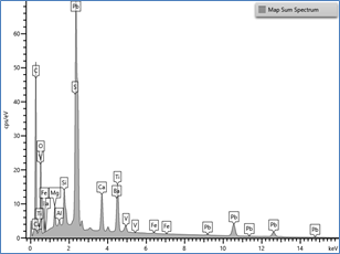
Fig. 1: Left – EDS X-ray spectrum. Right – EDS X-ray map layered on electron image. Which one is easier to understand the story of the paint sample?
With the release of the Ultim range of large area silicon drift detectors, laboratories can now communicate complex stories with efficiency via an image-centric workflow. Large area silicon drift detectors [40, 65, 100, and 170 (mm2)] paired with the low-noise X4 pulse processor powers the advanced software package AZtecLive.
AZtecLive has brought about a new age of image-based analysis. We can now begin with a live color image that transforms the first moments of investigative analysis into immediate results.
Fig. 2: AZtecLive software displays live spectrum, live X-ray maps, and live electron image.
Much like the way that we now watch TV, we no longer need to wait for results, or for the next episode of the image series. Instead, binge watching sample images has become the new norm. Moving sample to sample is now possible within minutes versus hours or even days. But how do we as scientists navigate the volumes of information at our fingertips? Choosing the correct citation, reading the best papers, and reporting the correct results have become more of a challenge as we produce more data.
1. Change Beam Energy
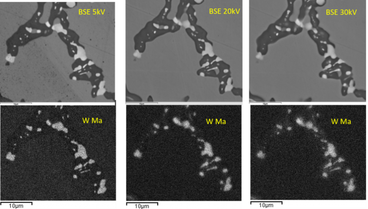
Instead of relying on one point of view, by exploring many we can enhance our understanding. Mapping at 20kV generates a large interaction volume that can spread the signal and may obscure grain boundaries, surface defects, and diffusion gradients. Collecting a second or third map at a lower energy such as 5 or 10kV can offer a fresh look at the same sample; we may see differences in grain boundaries, particle morphologies, and phase changes. With each new set of data, the picture becomes clearer, and we can feel more confident in the data reported.

Fig. 3: Top – BSE images collected at 5, 20, 30kV. Bottom – Tungten X-ray maps collected at 5, 20, 30kV. Images and maps from the Oxford Instruments NanoAnalysis EDS Applications Training Course.
2. Change Element Line Series in AZtec
We can also see through multiple points of view by changing the displayed element line series in AZtec Construct Maps. Atoms carry electrons in discrete energy states commonly known as “shells” and “orbits”. These energy states act as unique identifiers for each element in the periodic table. With elements that have more than one shell, they are labeled as K, L, M, etc. in descending order of energy. The K-shell has a higher ionization energy and therefore the X-rays have more energy than the L-shell X-rays (more energy is required to remove an electron from the K-shell than those shells further from the atomic nucleus).
When we think about X-ray spatial resolution, we must consider how far that X-ray can travel in the sample. The amount of energy that an X-ray has is directly proportional to its mean free path; higher energy has a larger interaction volume. Another factor are the other atoms in the sample; larger atoms have more stuff to absorb x-rays, smaller atoms have less stuff to absorb x-rays. This stuff can be defined as protons, neutrons, bosons, fermions, gluons, etc. The higher energy carries the X-rays further through a sample before they can escape and enter the EDS detector, or before they are absorbed by neighboring atoms. Sometimes the lower energy X-rays have more background under the curve and augment the apparent intensity. Changing the displayed line series of an element in a map, such as Pb L-alpha to the Pb M-alpha can show a different story.
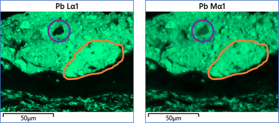
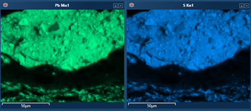
Fig. 4: Left – Pb Lα1 map higher energy X-rays have a longer mean free path and a deeper interaction volume, but less background intensity. Right – Pb Mα1map lower energy X-rays have a shorter mean free path and a smaller interaction volume, but more background intensity. Colors – The orange highlight shows effect of interaction volume. The purple highlight shows effect of lower background in L-alpha map.
Where the Lα1 X-rays move further in the sample we see a diffuse boundary and the Mα1 X-rays travel a shorter distance before being absorbed, therefore we see an image more representative of the surface of the sample (a smaller interaction volume and shorter mean free path).
3. Change Map Display to TruMap
Many samples contain two or more elements that share similar energy and overlap on the spectrum such as Lead/Sulfur and Barium/Titanium. The AZtec EDS map default is Window Integral Maps, pixels are colored according to energy windows. Since the two elements Pb/S share the same energy range they appear the same. Changing line series will not solve this problem since the low energy Sulfur Ll line is not visible above background. Earlier in our blog series Dr. Simon Burgess wrote about background subtracted maps. AZtecLive offers a one-button solution, TruMap, to separate artifacts from overlapping elements via deconvolution and to subtract fluctuations from background effects.
Fig. 5: Left – Highlighted Pb energy window (2.292-2.399keV) overlaps with S window (2.255-2.361keV). Right – Pb and S maps appear in the same location due to overlapping energy windows.
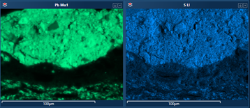
Fig. 6: Left – S Ll peak shape below background. Right – S Ll map still appears in same location as Pb Mα1.

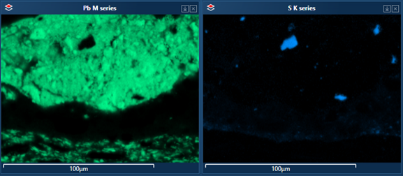
Fig. 7: Pb M series and S K series TruMaps, display the correct location of S via the applied algorithm deconvolution of overlapping peaks and reduced background fluctuations.
Hours, days, or years later when we want to revisit a sample, we can reconstruct the data from the original AZtec project. The entire data cube is saved per pixel. We can change line series in maps and quantification, apply TruMap or QuantMap, and even reconstruct spectra directly from the saved map data. AZtecLive delivers powerful tools to see through to the best answer. Discover how AZtecLive could allow you to better navigate and understand your samples.
Find out more